Using a multi-temperature dilatometry approach, you directly calculate activation energy by plotting the logarithm of the time to a fixed shrinkage against inverse temperature.
The core technique involves sintering identical powder compacts in a high-temperature dilatometer at several constant temperatures. From the shrinkage-versus-time curves, you extract the reciprocal of the time needed to reach a specific linear shrinkage value for each temperature. Plotting the natural log of that reciprocal time against the reciprocal absolute temperature (1/T) yields a straight line whose slope is ‑Q/R, giving the apparent activation energy (Q) for densification. This straight‑line Arrhenius behavior reveals the energy barrier of the dominant diffusion mechanism driving pore closure.
The apparent activation energy for powder densification is the slope of an Arrhenius plot constructed from high‑temperature furnace dilatometry data. By recording how fast the compact shrinks at multiple soak temperatures, you isolate the temperature‑dependent kinetics of the dominant mass‑transport process, enabling accurate prediction of density evolution during sintering.
Sintering as a Thermally Activated Process
Densification during sintering is not a simple melting event. It is a diffusion‑controlled process where atoms migrate to eliminate pores, and the rate at which this happens is exponentially sensitive to temperature.
The Arrhenius Relationship and Diffusion
The volume diffusion coefficient that governs mass transport follows D = D₀ exp(–Q/RT).
Here Q is the activation energy, R the universal gas constant, and T the absolute temperature.
Raising the furnace temperature dramatically increases atomic jump frequencies, accelerating neck growth and pore shrinkage.
Without sufficient thermal energy, atoms cannot overcome the energy barrier to move into vacant lattice sites.
The high‑temperature furnace supplies that energy, making Q a fundamental kinetic fingerprint of the powder system.
Why Activation Energy Matters
Knowing Q allows you to predict exactly how fast a compact will densify at any temperature profile.
This transforms furnace scheduling from an empirical trial‑and‑error process into a computationally optimized heating strategy.
For example, an accurate Q enables you to design a temperature ramp that reaches full density while minimizing grain growth and energy consumption.
The Direct Method: From Dilatometry to Arrhenius Plot
The most direct route to Q uses continuous shrinkage data from a high‑temperature push‑rod dilatometer.
The key is to run multiple isothermal holds and compare how the shrinkage–time curves translate with temperature.
Step 1: Collecting Constant‑Temperature Shrinkage Data
Identical green compacts are heated rapidly in the dilatometer to a series of target soak temperatures.
At each temperature, the system records linear shrinkage (ΔL/L₀) as a function of time under an inert or controlled atmosphere.
The result is a family of curves, each showing the time evolution of densification at a fixed temperature.
Step 2: Determining Time Exponent from Log‑Log Plots
For a given diffusion mechanism, the early‑stage shrinkage follows a power‑law relation with time.
By plotting ln(ΔL/L₀) versus ln(t) for each temperature, you can identify the time exponent that characterizes the dominant mechanism.
This check confirms that the densification kinetics are self‑similar and that a meaningful single activation energy can be defined.
Step 3: Constructing the Arrhenius Plot (1/t vs 1/T)
This is the core calculation. For a chosen constant shrinkage value (e.g., y = 1%), read the time t required to reach that shrinkage from each curve.
Take the reciprocal time (1/t) as a rate measure, and plot ln(1/t) against 1/T.
Because the rate is proportional to exp(–Q/RT), the slope of this line equals –Q/R. Multiply by R and take the absolute value to obtain Q.
A Worked Example from Metal Powder Compacts
For micro‑scale metal powder compacts sintered across several high‑temperature holds, this method yields activation energies in the range of 291.3 kJ/mol to 309 kJ/mol.
These values correspond to grain‑boundary or volume diffusion dominating densification, depending on the temperature window.
The straight‑line Arrhenius fit validates that a single diffusion mechanism controls the process under those conditions.
Modern Techniques: Master Sintering Curve (MSC) and Residual Minimization
While the direct isothermal method is foundational, many modern labs use constant heating rate (CHR) experiments and mathematical fitting to extract Q from a single densification master curve.
The Master Sintering Curve Concept
The MSC collapses all density–temperature–time data from different heating rates onto a single curve.
This is possible because densification follows a work‑of‑sintering parameter θ that integrates temperature history with the unknown Q.
By varying Q in the integration, you find the value that best superposes all experimental density points onto one smooth master line.
Curve Fitting and Minimizing Residuals for Q
First, a sigmoidal or polynomial function is fitted to the empirical density data to create a smooth reference curve.
Then the mean square residual between the fitted curve and the MSC‑predicted density is calculated for a range of trial Q values.
The Q that gives the lowest residual is taken as the apparent activation energy. This global approach uses all available data, reducing sensitivity to single‑point noise.
Essential Role of High‑Temperature Furnace Control
The fidelity of your Q value is entirely limited by the quality of your thermal data.
The Criticality of Linear Heating Ramps
Constant‑heating‑rate MSC methods require exceptionally stable, repeatable ramps, often 5‑20 °C/min up to 1500 °C or higher.
Any furnace overshoot, lag, or non‑linearity distorts the shrinkage‑rate curves and corrupts the θ integral.
Laboratory‑grade furnaces with PID feedback and calibrated thermocouples must be used.
Precise Thermal Logging and the Thermal Parameter θ
The parameter θ = ∫₀ᵗ exp(–Q/RT(t)) dt is numerically integrated using the logged temperature‑time history.
Even small errors in measured sample temperature introduce significant errors in θ, causing the residual‑minimization to converge on a false Q.
Direct sample‑contact thermocouples and regular calibration are not optional extras—they are prerequisites for meaningful kinetic analysis.
Understanding the Trade‑offs
No single method is universally perfect, and practitioners must recognize where the standard approaches break down.
Assumption of a Single Dominant Mechanism
The Arrhenius and MSC methods implicitly assume that one diffusion mechanism governs densification over the entire temperature range.
If the dominant mechanism shifts—from grain‑boundary diffusion at intermediate temperatures to lattice diffusion near the end—a single Q becomes an oversimplification.
The resulting apparent activation energy will be an averaged value that may not accurately predict behavior outside the calibration range.
Sensitivity to Measurement Accuracy and Grain Growth Interference
Dilatometry measures macroscopic linear shrinkage, not directly density. Anisotropic shrinkage or thermal expansion drift can bias the data.
At high soak temperatures, grain growth can accelerate and alter the density‑time trajectory independently of the densification mechanism.
This causes a deviation from the pure kinetics assumed, making the extracted Q less reliable if the soak is too long or too hot.
Applicability to Constant Rate vs Isothermal Conditions
The direct isothermal method requires a physically meaningful fixed shrinkage target and assumes negligible densification during heat‑up.
In contrast, MSC techniques harvest information from the entire heating and cooling history, making them robust to small heat‑up effects.
However, MSC fits can be sensitive to the functional form chosen for the master curve, introducing a user‑dependent bias.
Making the Right Choice for Your Process Optimization
The best method depends on your equipment, your powder’s thermal history, and how you plan to use the Q value.
- If your primary focus is quick screening of multiple powder batches: Use the direct isothermal method with a single fixed‑shrinkage target and three to four soak temperatures. It delivers a reliable apparent activation energy without complex numerical fitting.
- If your primary focus is building a predictive sintering model across variable heating profiles: Apply the Master Sintering Curve residual‑minimization technique to constant‑heating‑rate runs at three or more ramp rates. The resulting Q will support accurate θ‑based predictions.
- If your primary focus is pressure‑assisted or field‑assisted sintering: Be aware that electric currents and mechanical pressure can lower the apparent Q dramatically. Extract Q from creep‑based densification models rather than pressureless sintering kinetics to capture the true rate‑controlling mechanism.
- If your primary focus is scaling from lab to production furnaces: Validate the lab‑derived Q by comparing predicted density–time trajectories with data from a pilot‑scale furnace that mimics your production thermal profile. This ensures the kinetic parameters transfer across equipment.
The activation energy extracted from careful high‑temperature furnace thermal analysis transforms a black‑box sintering cycle into a designed, efficient pathway to full density.
Summary Table:
| Method | Experimental Input | Key Plot / Calculation | Best Used For |
|---|---|---|---|
| Direct Isothermal | Shrinkage vs. time at multiple fixed temperatures | Slope of ln(1/t) vs. 1/T yields -Q/R | Quick screening & single shrinkage targets |
| Master Sintering Curve (MSC) | Shrinkage vs. temperature at multiple heating rates | Minimizing mean square residual of thermal parameter (θ) | Robust predictive modeling across complex thermal cycles |
| Creep-Based Densification | Continuous shrinkage under external pressure or field | Strain rate equations tailored to stress/field | Pressure-assisted or electric field-assisted sintering |
Achieve Precise Thermal Control for Accurate Sintering Kinetics with KINTEK
Extracting reliable activation energy requires precise thermal logging, uniform heating profiles, and ultra-stable temperature control. KINTEK specializes in advanced laboratory equipment and high-temperature furnaces designed to meet rigorous research standards.
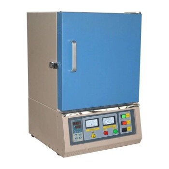
From muffle, tube, and rotary furnaces to high-vacuum, atmosphere-controlled, CVD, dental, and induction melting systems, all of our high-temperature solutions can be fully customized to your specific powder processing and dilatometry requirements.
Don't let furnace fluctuations compromise your kinetic data. Contact KINTEK today to consult with our thermal processing experts and find the ideal furnace for your laboratory!
Related Products
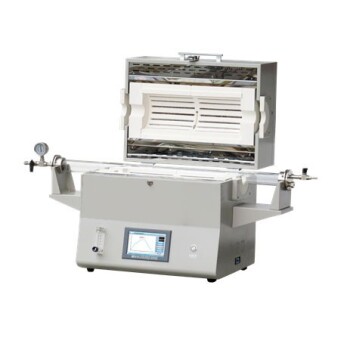
- 1400℃ High Temperature Laboratory Tube Furnace with Alumina Tube
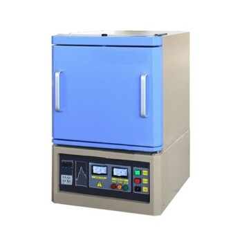
- 1800℃ High Temperature Muffle Oven Furnace for Laboratory
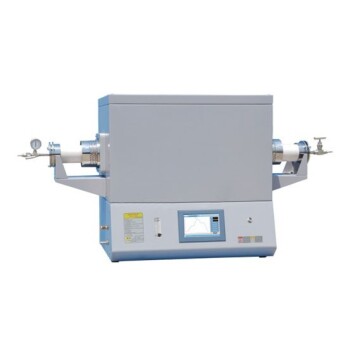
- 1700℃ High Temperature Laboratory Tube Furnace with Alumina Tube
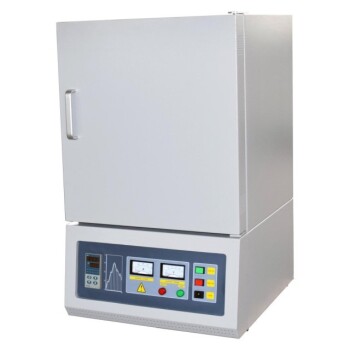
- 1700℃ High Temperature Muffle Oven Furnace for Laboratory
- 1200℃ Muffle Oven Furnace for Laboratory
People Also Ask
- How does zone-melting in tube furnaces synthesize bismuth micro-wires? Master Single-Crystal Thermoelectric Growth
- How are high-temperature laboratory tube furnaces applied in long-term vacuum homogenization heat treatments for intermetallic samples?
- How do high-temperature laboratory tube furnaces ensure environmental stability? Precision Thermal Reduction Tips
- How are high-temp tube furnaces used to measure diffusion coefficients per Fick's law? Master Precision Annealing
- How are high-temperature tube furnaces applied in testing ceramic-supported alloy membranes? Insights